Simulate Refractive Scattering

Another feature of ScatteringOptics.jl is simulating refractive scattering. This page gives a tutorial to simulate refractive scattering effects.

Loading your image

Again, we use an example image in eht-imaging. Data can be downloaded from here (please open in a new window. otherwise you will get 404 error). This is a general relativistic magnetohydrodynamic (GRMHD) model of the magnetic arrestic disk originally from Dexter et al. 2014.

using CairoMakie
# This is the base package for the Skymodel of the Comrade.jl ecosystem
using VLBISkyModels
# Alternatively, you can import Comrade.jl instead. Either works.
# using Comrade

# Load a image model from an image FITS file
im = load_fits("data/jason_mad_eofn.fits", IntensityMap)

# Frequency of the image
νref = metadata(im).frequency
print("Frequency of the image: ", νref/1e9," GHz")

# Plot source image
imageviz(im, size=(600, 500), colormap=:afmhot)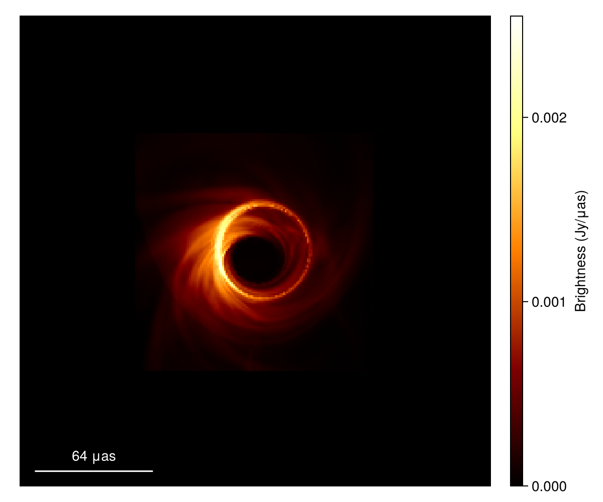

Simulating Refractive Scattering

And, then again initialize a scattering model.

using ScatteringOptics

# initialize the scattering model
sm = ScatteringModel()

DipoleScatteringModel{Float64}(1.38, 8.0e7, 1.38, 0.703, 81.9, 1.0, 8.701673999999999e21, 1.7063921e22, 0.5099457504520795, 0.5879203321591805, 1.9630156472261735, 3.8933699749663195, 10.476370590888147, 3.5025254191248507, 4.04238102210397e19, 5.8567426819253905, 4.650020392426908, 1.2067222894984828, 0.14137166941154058, 27.969627943900058, 0.24094564298608265, 16.43371800974761, 0.10641979388314901, 0.5127694683107693)

Refractive scattering will distort the diffractively-scattered (i.e. emsemble-average) image and add compact substrucures so-called refractive substructures. These effects will be simulated with a phase screen generated from the probabilistic magnetic field wander model of the intersteller medium implemented in the scattering model.

First, let's initialize a phase screen model (RefractivePhaseScreen) from the scattering model and the model image.

# Initialize a refractive phase screen model from scattering and image models
rps = refractivephasescreen(sm, im)

# Alternatively, you may make the screen model for arbitral grid
#   ScatteringOptics is design to work even if ScatteringScreen's grid is not consistent
#   with the image you want to scatter, thanks to a powerful interpolation scheme available.
# rps = RefractivePhaseScreen(sm, Nx, Ny, dx_rad, dy_rad)

RefractivePhaseScreen{DipoleScatteringModel{Float64}, Float64, StationaryRandomFields.NoiseSignal, PhaseScreenPowerLaw{2, DipoleScatteringModel{Float64}, Float64}}(DipoleScatteringModel{Float64}(1.38, 8.0e7, 1.38, 0.703, 81.9, 1.0, 8.701673999999999e21, 1.7063921e22, 0.5099457504520795, 0.5879203321591805, 1.9630156472261735, 3.8933699749663195, 10.476370590888147, 3.5025254191248507, 4.04238102210397e19, 5.8567426819253905, 4.650020392426908, 1.2067222894984828, 0.14137166941154058, 27.969627943900058, 0.24094564298608265, 16.43371800974761, 0.10641979388314901, 0.5127694683107693), 4.218690603755095e10, 4.218690603755095e10, StationaryRandomFields.NoiseSignal{Tuple{Int64, Int64}}((256, 256)), PhaseScreenPowerLaw{2, DipoleScatteringModel{Float64}, Float64}(DipoleScatteringModel{Float64}(1.38, 8.0e7, 1.38, 0.703, 81.9, 1.0, 8.701673999999999e21, 1.7063921e22, 0.5099457504520795, 0.5879203321591805, 1.9630156472261735, 3.8933699749663195, 10.476370590888147, 3.5025254191248507, 4.04238102210397e19, 5.8567426819253905, 4.650020392426908, 1.2067222894984828, 0.14137166941154058, 27.969627943900058, 0.24094564298608265, 16.43371800974761, 0.10641979388314901, 0.5127694683107693), 4.218690603755095e10, 4.218690603755095e10, 0.0, 0.0))

You can sample a Gaussian noise in the Fourier domain.

# Generate a phase screen. For this particular tutorial we will use StableRNG for the reproducibility.
using StableRNGs
rng = StableRNG(123)
noise_screen = generate_gaussian_noise(rps; rng=rng)

129×256 Matrix{ComplexF64}:
        0.0+0.0im        -1.42237+0.211806im     …    -0.14404-1.46535im
   0.471559+1.23739im    0.660122+0.0873872im         -0.54038-0.185399im
  -0.888559-0.219822im  -0.476492+0.793291im         -0.614426-1.14927im
  -0.060101+0.194956im   0.185724+0.00740253im       0.0029722+0.315275im
 -0.0666618-0.12437im   -0.313947-0.317471im         -0.659719+0.615051im
   0.691469-0.418463im  -0.229056+0.436795im     …  -0.0913364-1.38856im
   -0.47423-1.34245im     1.15835-1.36531im          -0.487128-0.136273im
  -0.505398-0.145882im   0.472817-0.502366im         -0.768268-0.5478im
  -0.683912+0.158674im   -1.26309+0.77461im           0.677391-0.3282im
  -0.964627-0.33336im     0.53031-1.0641im          -0.0528775-0.864448im
           ⋮                                     ⋱            ⋮
   -1.21983+0.583945im  -0.683662+0.615531im     …    0.513594+0.723873im
   0.094109+0.206076im  0.0302826+0.15087im            -1.0777+0.49935im
   0.549581+0.862441im  -0.288871+0.719656im          0.717905-0.790146im
  -0.283655+0.505174im  -0.451472+0.0615803im         0.645413-0.971754im
 -0.0350022-1.03477im    -1.21324-0.15738im          -0.142354-0.245928im
   0.470806+0.257644im  -0.713483+0.000997682im  …   0.0947333+1.46063im
    0.34574-1.17356im     0.33842+0.00476794im       0.0671579-0.676809im
  -0.625574-0.668117im  -0.784044+0.289585im          0.440891-0.59245im
   -1.18389+0.0im       -0.771524+1.35287im            0.50275-0.443054im

This Gaussian noise will be scaled with the powerspectrum of the phase screen, and then transformed into the actual phase screen. The fully scattered image can be generated by scatter_image method.

# Produce the scattered image
im_a = scatter_image(rps, im; noise_screen=noise_screen)

# Plot source image
imageviz(im_a, size=(600, 500), colormap=:afmhot)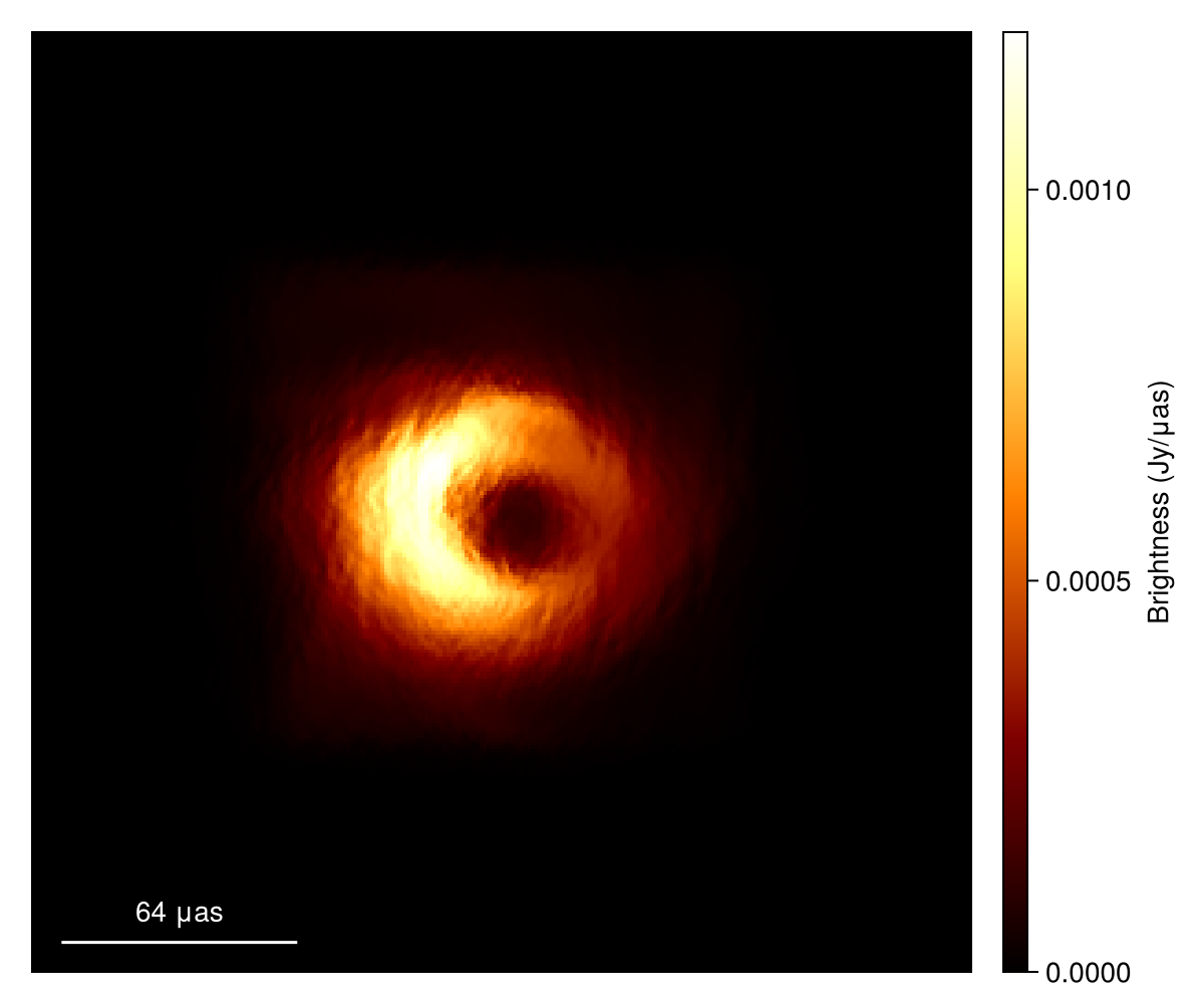

If you completely randomize the process, you can skip the step to generate noise_screen and specify it in the argument of scatter_image method. In this case, the screen will be automatically generated inside scatter_image method.

There is a quick shortcut bypassing the noise screen generation, which has a less flexibility and a larger overhead for iterative processes.

# Produce scattered image with observing wavelength .13 cm
im_a2 = scatter_image(sm, im; rng=rng)

# Plot source image
imageviz(im_a2, size=(600, 500), colormap=:afmhot)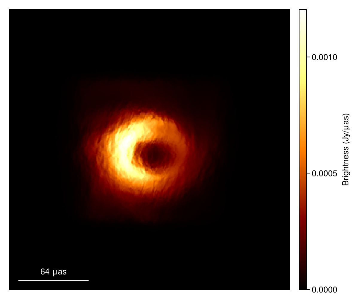

Just because the refractive scattering effects cannot be described analytically in Fourier domain, scatter_image method only works for the image models (::IntensityMap). For sky models in VLBISkyModels.jl, you need to first instantiate an image model of your sky model.

Here we show an example using a simple Gaussian model. You need to create an image model with intensitymap method from VLBISkyModels.jl.

# Gaussian model from VLBISkyModels.jl
g = stretched(Gaussian(), μas2rad(5.0), μas2rad(5.0))

# Create an image model from the Gaussian model
im_g = intensitymap(g, imagepixels(μas2rad(200.0), μas2rad(200.0), 256, 256))

# Plot source image
imageviz(im_g, size=(600, 500), colormap=:afmhot)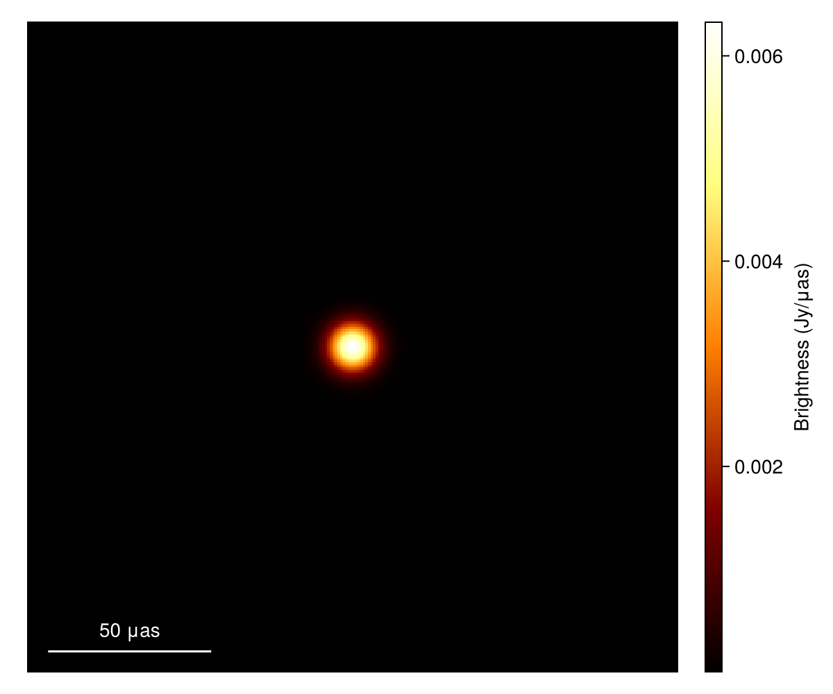

Then you can make a scattered image. Don't forget to add the observing frequency as im_g doesn't have a frequency information.

# Produce scattered image. Don't forget to add the observing frequency as im_g doesn't have a frequency information.
im_ga = scatter_image(sm, im_g; rng=rng, νref=νref)

# Plot source image
imageviz(im_ga, size=(600, 500), colormap=:afmhot)

Save the tutorial data and do some unit tests

The output images may be saved to fits files. Here, we save the images generated in the tutorial above.

# Average image of provided EHT fits file
save_fits("data/im_a.fits", im_a)
# Scattered average image of Gaussian model
save_fits("data/im_ga.fits", im_ga)

The saved files are available here (im_a.fits, im_ga.fits; please open in a new window. otherwise you will get 404 error).

Unit Tests

Julia codes in our tutorial are automatically run at the compilation of the documentation at GitHub Workflow, and therefore those files are kept produced with the corresponding version of the package. For your own unit tests, you can compare fits files created in your local enviroment with these reference data. For instance, for the images,

im_a_ref = load_fits("downloaded im_a.fits", IntensityMap)

# take differences
Δim_a = im_a .- im_a_ref

# compute a fractional error map
fim_a = Δim_a ./ (im_a_ref .+ 1e-10)

# plot the error map
imageviz(abs.(fim_a))

In our tests, which compare images produced at GitHub (using ubuntu and x86 architecture) and a computer of the developer members (macOS with Apple Silicon M3 architecture), the maximum and mean fractional errors were $\sim {10}^{-8}$ (found at the edge of images where the intensity is almost 0) and $\sim {10}^{-13}$, respectively. This is a sufficient accuracy for the vast majority (if not all!) of the analysis done in the EHT and broader radio astronomy communities.