Simulate Diffractive Scattering
ScatteringOptics.jl is designed as a package inside the ecosystem of Comrade.jl. The scattering model in the package can scatter any sky model types from Comrade.jl. This page describes how to simulate diffractive scattering.
Loading your image
Here, we use an example image in eht-imaging. Data can be downloaded from here (please open in a new window. otherwise you will get 404 error). This is a general relativistic magnetohydrodynamic (GRMHD) model of the magnetic arrestic disk originally from Dexter et al. 2014.
using CairoMakie
# This is the base package for the Skymodel of the Comrade.jl ecosystem
using VLBISkyModels
# Alternatively, you can import Comrade.jl instead. Either works.
# using Comrade

# Load a image model from an image FITS file
im = load_fits("data/jason_mad_eofn.fits", IntensityMap)

# Plot source image
imageviz(im, size=(600, 500), colormap=:afmhot)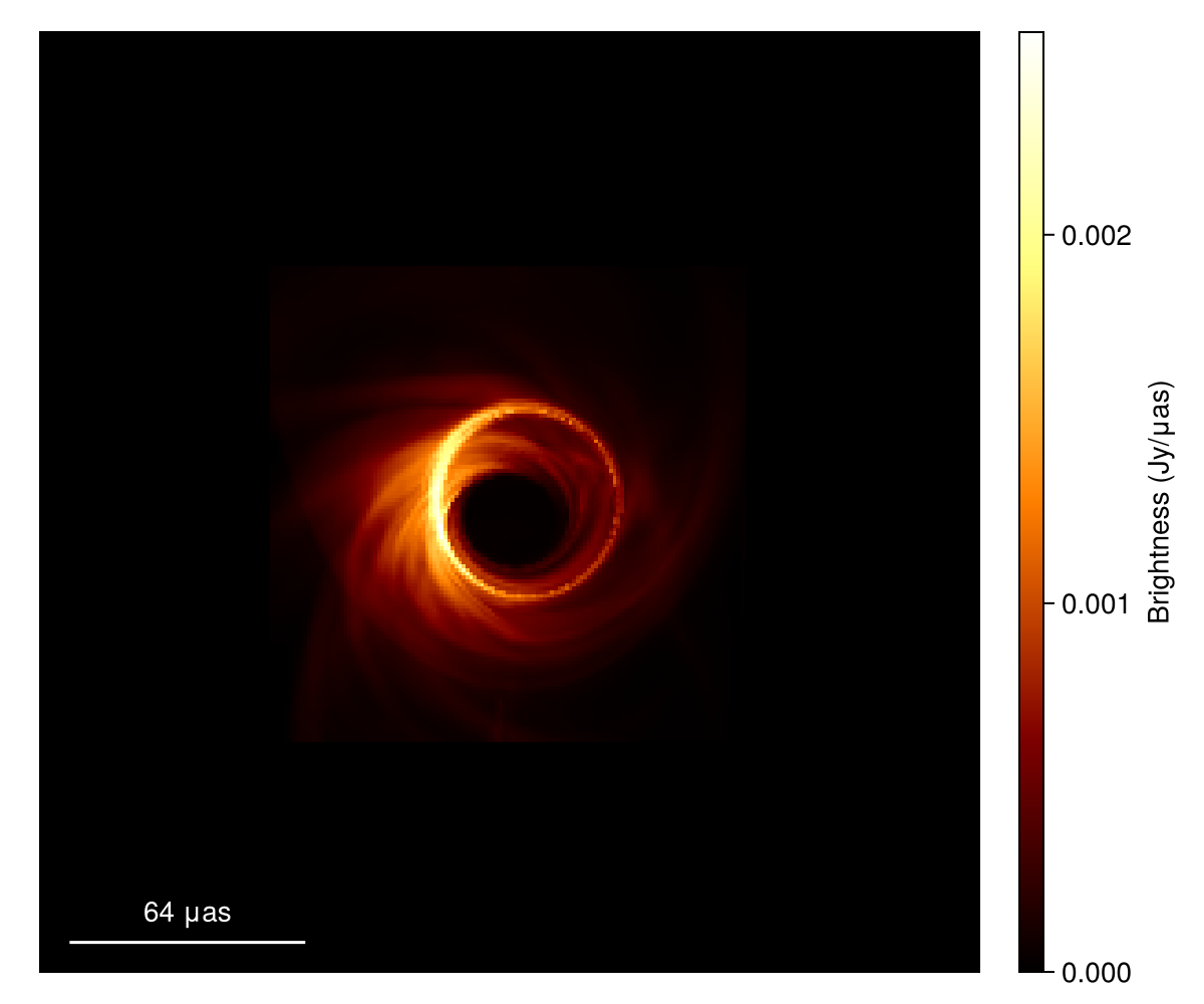
You can instantiate your scattering model with ScatteringModel(). If nothing is specified, the model will use the best-fit parameter set for Sgr A* in Johnson et al. 2018.
using ScatteringOptics

# initialize the scattering model
sm = ScatteringModel()
DipoleScatteringModel{Float64}(1.38, 8.0e7, 1.38, 0.703, 81.9, 1.0, 8.701673999999999e21, 1.7063921e22, 0.5099457504520795, 0.5879203321591805, 1.9630156472261735, 3.8933699749663195, 10.476370590888147, 3.5025254191248507, 4.04238102210397e19, 5.8567426819253905, 4.650020392426908, 1.2067222894984828, 0.14137166941154058, 27.969627943900058, 0.24094564298608265, 16.43371800974761, 0.10641979388314901, 0.5127694683107693)You can change the parameters if you want to simulate a different scattering screen. See ScatteringOptics.DipoleScatteringModel for arguments.
Simulate diffractive scattering
As explained in Brief Introduction to Interstellar Scattering, diffractive scattering will cause angular broaderning of the resultant image, which is described by the convolution of the source image with a scattering kernel. ScatteringOptics.jl implements a Comrade.jl's skymodel of the scattering kernel. You can generate it by
# Frequency of the image
νref = metadata(im).frequency
print("Frequency of the image: ", νref/1e9," GHz")

# Create kernel from scattering model
skm = kernelmodel(sm, νref=νref)
ApproximatedScatteringKernel{Float64, DipoleScatteringModel{Float64}, Float64}(DipoleScatteringModel{Float64}(1.38, 8.0e7, 1.38, 0.703, 81.9, 1.0, 8.701673999999999e21, 1.7063921e22, 0.5099457504520795, 0.5879203321591805, 1.9630156472261735, 3.8933699749663195, 10.476370590888147, 3.5025254191248507, 4.04238102210397e19, 5.8567426819253905, 4.650020392426908, 1.2067222894984828, 0.14137166941154058, 27.969627943900058, 0.24094564298608265, 16.43371800974761, 0.10641979388314901, 0.5127694683107693), 2.29345e11)skm is a subtype of ComradeBase.AbstractModel, and you can use any methods defined for sky models in Comrade.jl's ecosystem. For instance, you can compute the ensemble-average (or diffractively scattered) image using the convolve method from VLBISkyModels.jl,
# scatter the image
im_ea = convolve(im, skm)

# Plot source image
imageviz(im_ea, size=(600, 500), colormap=:afmhot)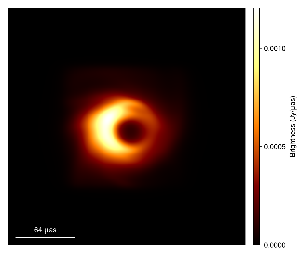
You can also directly convolve a skymodel from ComradeBase.AbstractModel and implemented in VLBISkyModels.jl.
# Gaussian model from VLBISkyModels.jl
g = stretched(Gaussian(), μas2rad(5.0), μas2rad(5.0))
im_g = intensitymap(g, imagepixels(μas2rad(200.0), μas2rad(200.0), 256, 256))

# Plot source image
imageviz(im_g, size=(600, 500), colormap=:afmhot)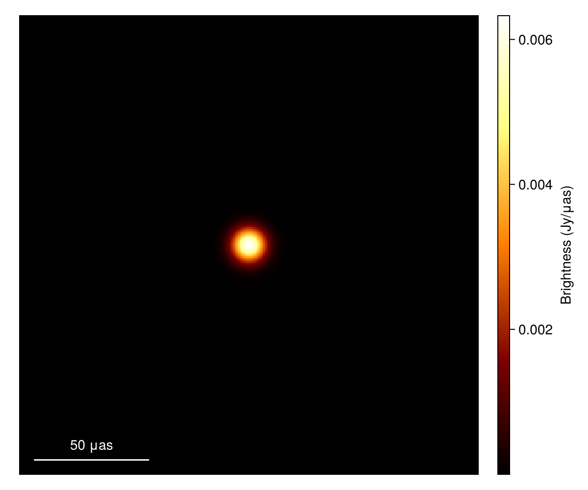
Scattered model and image can be generated by,
g_ea = convolved(g, skm)
im_gea = intensitymap(g_ea, imagepixels(μas2rad(200.0), μas2rad(200.0), 256, 256))

# Plot source image
imageviz(im_gea, size=(600, 500), colormap=:afmhot)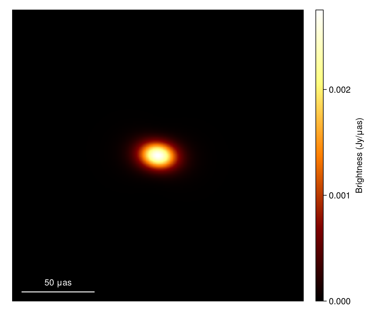
You can also plot the scattering kernel. For instance in the image domain,
# make an image model of the scattering kernel
im_skm = intensitymap(skm, imagepixels(μas2rad(50.0), μas2rad(50.0), 256, 256))

# Plot source image
imageviz(im_skm, size=(600, 500), colormap=:afmhot)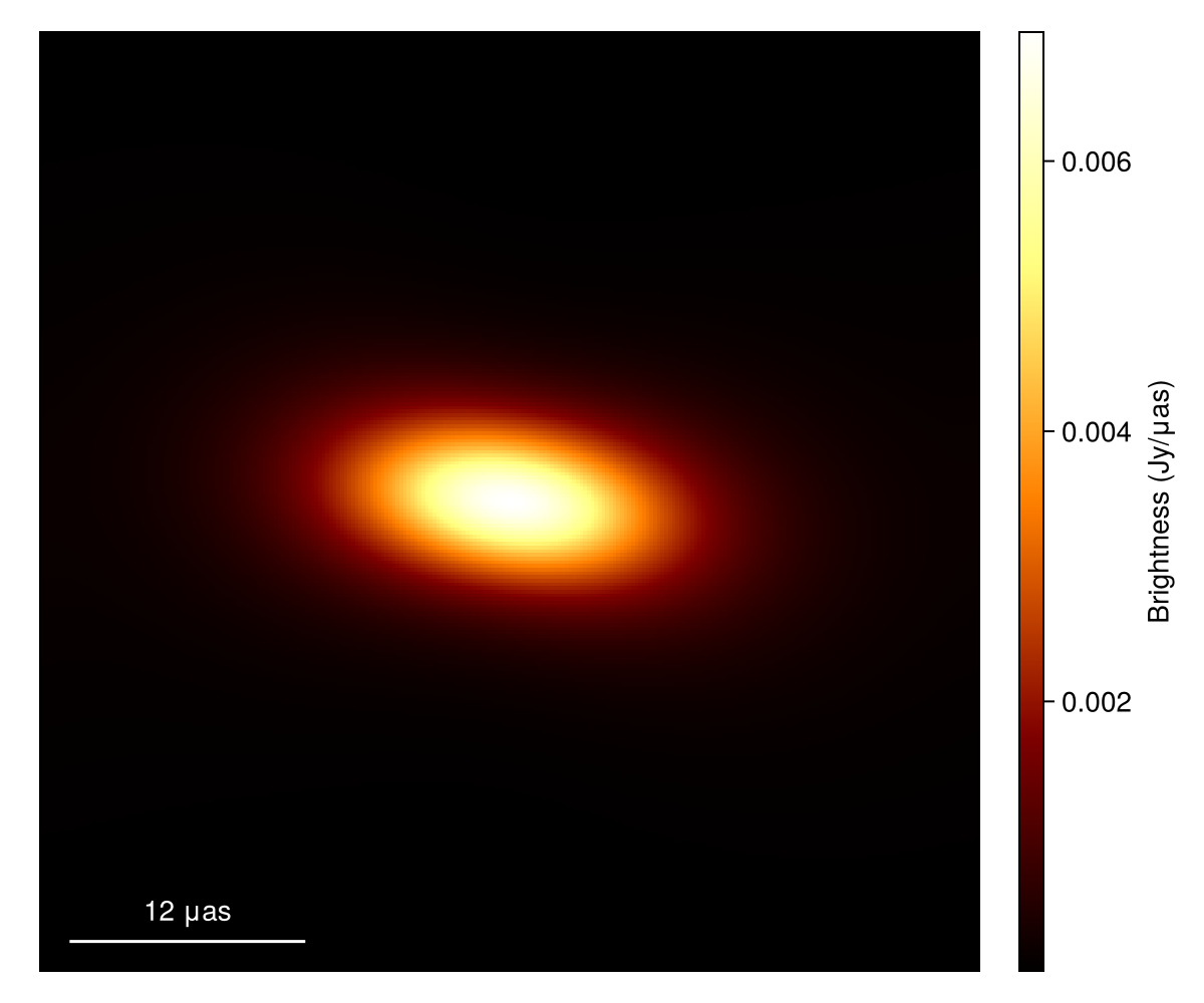
You can compute the kernel visibility using visibility_point method from VLBISkyModels.jl. For instance,
# computing kernels from 0 to 10 Glambda along RA
u = LinRange(0,10e9,1000)
vis = [visibility_point(skm, (U=u, V=0, Fr=νref)) for u=u]

# Plot source image
f = Figure()
ax = Axis(f[1, 1],
    xlabel="Baseline Length (Gλ)",
    ylabel="Kernel Amplitudes",
)
plot!(ax, u/1e9, abs.(vis))
f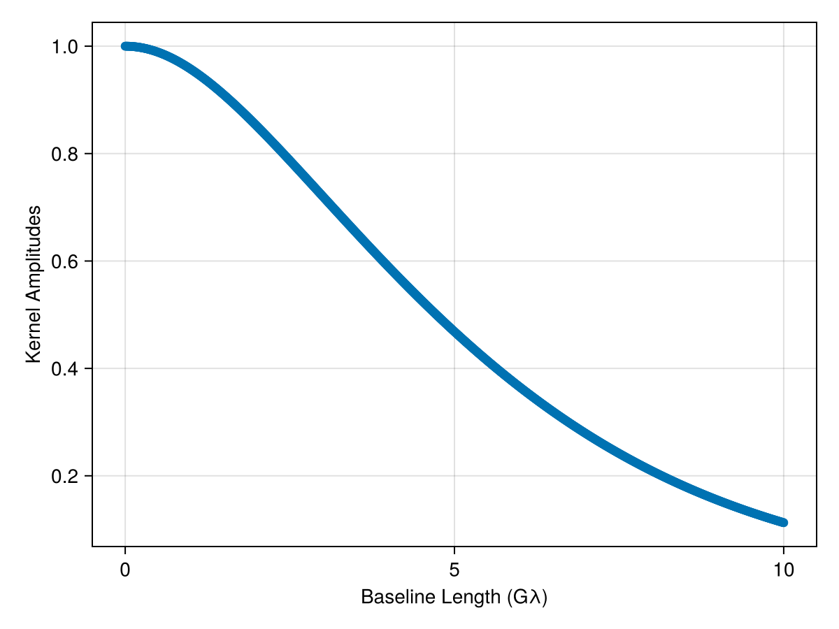
A quick shortcut
The above tutorial is intentionally written in a low level. There is ensembleaverage method to do a quick shortcut by bypassing the kernel generation.
# scatter the image
im_ea_2 = ensembleaverage(sm, im)

# Plot source image
imageviz(im_ea_2, size=(600, 500), colormap=:afmhot)
Although this is handy, it may have an extra overhead to initialize skm which may slow down highly iterative processes. ensembleaverage method also supports more general skymodels in ComradeBase.AbstractModel as an input instead of the image model.
Save the tutorial data
The output images may be saved to fits files. Here, we save the images generated in the tutorial above.
# Ensemble average image of provided EHT fits file
save_fits("data/im_ea.fits", im_ea)
# Gaussian model and its scattered ensemble average image
save_fits("data/im_g.fits", im_g)
save_fits("data/im_gea.fits", im_gea)
# Scattering kernel
save_fits("data/im_skm.fits", im_skm)
You can download generated files from here (im_ea.fits, im_g.fits, im_gea.fits, im_skm.fits; please open in a new window. otherwise you will get 404 error).
We also save the kernel visibilities calculated in the tutorial.
using HDF5

# Save the computed kernel data
h5open("data/kernel.h5", "w") do file
    file["u"] = collect(u)
    file["vis"] = vis
end
1000-element Vector{ComplexF64}:
1.0 + 0.0im
0.9999954071523528 + 0.0im
0.9999816289767681 + 0.0im
0.9999586665751884 + 0.0im
0.9999265217837584 + 0.0im
0.9998851971721843 + 0.0im
0.9998346960428404 + 0.0im
0.9997750224296191 + 0.0im
0.9997061810965293 + 0.0im
0.9996281775360422 + 0.0im
⋮
0.11559473637711046 + 0.0im
0.11522330025187441 + 0.0im
0.11485290794090472 + 0.0im
0.11448355715840004 + 0.0im
0.11411524562062209 + 0.0im
0.11374797104590981 + 0.0im
0.11338173115469348 + 0.0im
0.11301652366950847 + 0.0im
0.11265234631500975 + 0.0imYou can find the generated file from here (please open in a new window. otherwise you will get 404 error). Additionally, for accuracy and speed evaluations of the scattering kernel, see Benchmarks.
Unit Tests
You can do your own unit tests by comparing your own outputs with those created in the website. Please see at the end of Simulate Refractive Scattering for a quick example.