Tutorial
This example code segment uses StationaryRandomFields.jl to generate correlated noise for a signal of given dimensions.
We begin by defining a noise signal object with dimensions input as a tuple.
using StationaryRandomFields
using FFTW

# Define a 2D signal with dimensions (1000,1000)
signal = NoiseSignal((1000,1000))
NoiseSignal{Tuple{Int64, Int64}}((1000, 1000))We can immediately access the RFFT frequency grid that corresponds to the signal dimensions
ν = rfftfreq(signal)([0.0, 0.001, 0.002, 0.003, 0.004, 0.005, 0.006, 0.007, 0.008, 0.009000000000000001 … 0.491, 0.492, 0.493, 0.494, 0.495, 0.496, 0.497, 0.498, 0.499, 0.5], [0.0, 0.001, 0.002, 0.003, 0.004, 0.005, 0.006, 0.007, 0.008, 0.009000000000000001 … -0.01, -0.009000000000000001, -0.008, -0.007, -0.006, -0.005, -0.004, -0.003, -0.002, -0.001])We can also directly create Gaussian noise in Fourier space for the given signal with an optional input of the desired rng (if not the default). This is not a necessary step as the NoiseGenerator will implement it automatically later.
gnoise = generate_gaussian_noise(signal)501×1000 Matrix{ComplexF64}:
0.0+0.0im -0.269552-0.429813im … 1.41428-0.482105im
-0.830418-0.26426im -1.87363+1.50812im -0.576537-0.310449im
-0.244077-0.532124im -0.0442435+0.983915im -0.103151+0.962699im
0.181734+0.22135im -1.13062+0.963826im 0.108631+0.800489im
-1.28894-1.30904im 0.0404853-0.229014im 0.298692-0.730373im
0.847101+0.047284im 0.595183-0.520453im … 0.115357+0.325241im
-0.393936-1.21027im -0.192824-0.44689im -0.773383+0.678284im
0.586405+0.815886im -0.35529+0.299089im 0.0429231-0.368123im
0.371949+0.371633im -1.07715+0.854258im 1.08109+0.307125im
-0.626764-0.553526im 0.59381-2.06708im 0.177241+0.123983im
⋮ ⋱
0.0306097-0.515289im -0.198415+1.12139im -0.746693-0.935851im
0.277608+0.398337im -0.0983214-0.0822972im 0.974913-0.113061im
-1.14263+0.61695im -0.0133414+0.788364im -0.345254-0.186545im
0.387461+0.354029im 0.864576+1.22085im … 0.564244-1.00237im
-0.182351+0.1848im 0.847312+1.04999im -0.143567-0.520828im
0.634817-0.744711im -0.995675-0.0875825im -0.456667+0.99535im
0.974676+0.213044im 0.616495+1.09545im 0.780201-0.353582im
-1.08735+1.07079im 0.249308+0.0541121im -0.0427284-0.36255im
-0.312939+0.0im 0.47319+1.2115im … -0.141857-0.758465imNow construct the power spectrum to be used, designating the dimension in brackets.
# Create a basic power spectrum with index β = -2
ps = SinglePowerLaw{2}(-2.)
SinglePowerLaw{2, Float64}(-2.0)The power spectrum may be modified via renormalization, rotation, and stretching
renormed_ps = 1000 * ps
rotated_ps = rotated(renormed_ps, π/6) # π/6 is the rotation factor
stretched_ps = stretched(rotated_ps, 100, 100) # 100 is the stretch factor of both axes
ModifiedPowerSpectrumModel
base model: SinglePowerLaw{2, Float64}
Modifiers:
1. Renormalize{Int64}
2. Rotate{Float64}
3. Stretch{Int64, 2}The noise generator requires a ContinuousNoiseSignal as input, which can be created from the original NoiseSignal
cns = ContinuousNoiseSignal(signal)ContinuousNoiseSignal{Float64, NoiseSignal{Tuple{Int64, Int64}}, Tuple, FFTW.rFFTWPlan{Float64, -1, false, 2, Tuple{Int64, Int64}}, AbstractFFTs.ScaledPlan{ComplexF64, FFTW.rFFTWPlan{ComplexF64, 1, false, 2, Tuple{Int64, Int64}}, Float64}}(NoiseSignal{Tuple{Int64, Int64}}((1000, 1000)), (1000, 1000), FFTW real-to-complex plan for 1000×1000 array of Float64
(rdft2-rank>=2/1
(rdft2-vrank>=1-x1000/1
(rdft2-ct-dit/20
(hc2c-direct-20/76/0 "hc2cfdftv_20_avx2"
(rdft2-ct-dit/2
(hc2c-direct-2/4/0 "hc2cfdftv_2_avx2"
(rdft2-r2hc-direct-2 "r2cf_2")
(rdft2-r2hc01-direct-2 "r2cfII_2"))
(dft-direct-10 "n1fv_10_avx2_128"))
(rdft2-r2hc01-direct-20 "r2cfII_20"))
(dft-vrank>=1-x10/1
(dft-ct-dit/5
(dftw-direct-5/4 "t3fv_5_avx2_128")
(dft-direct-10-x5 "n2fv_10_avx2_128")))))
(dft-buffered-1000-x32/501-6
(dft-vrank>=1-x32/1
(dft-ct-dit/25
(dftw-direct-25/8 "t3fv_25_avx2_128")
(dft-vrank>=1-x25/1
(dft-ct-dit/5
(dftw-direct-5/4 "t3fv_5_avx2_128")
(dft-direct-8-x5 "n2fv_8_avx2_128")))))
(dft-r2hc-1
(rdft-rank0-tiledbuf/2-x32-x1000))
(dft-buffered-1000-x21/21-6
(dft-vrank>=1-x21/1
(dft-ct-dit/25
(dftw-direct-25/8 "t3fv_25_avx2_128")
(dft-vrank>=1-x25/1
(dft-ct-dit/5
(dftw-direct-5/4 "t3fv_5_avx2_128")
(dft-direct-8-x5 "n2fv_8_avx2_128")))))
(dft-r2hc-1
(rdft-rank0-tiledbuf/2-x21-x1000))
(dft-nop)))), 1.0e-6 * FFTW complex-to-real plan for 501×1000 array of ComplexF64
(rdft2-rank>=2/1
(rdft2-vrank>=1-x1000/1
(rdft2-ct-dif/20
(hc2c-direct-20/76/0 "hc2cbdftv_20_avx2"
(rdft2-ct-dif/2
(hc2c-direct-2/4/0 "hc2cbdftv_2_avx2"
(rdft2-hc2r-direct-2 "r2cb_2")
(rdft2-hc2r10-direct-2 "r2cbIII_2"))
(dft-direct-10 "n1bv_10_avx2_128"))
(rdft2-hc2r10-direct-20 "r2cbIII_20"))
(dft-vrank>=1-x10/1
(dft-ct-dit/5
(dftw-direct-5/4 "t3bv_5_avx2_128")
(dft-direct-10-x5 "n1bv_10_avx2_128")))))
(dft-buffered-1000-x32/501-6
(dft-vrank>=1-x32/1
(dft-ct-dit/25
(dftw-direct-25/8 "t3bv_25_avx2_128")
(dft-vrank>=1-x25/1
(dft-ct-dit/5
(dftw-direct-5/4 "t3bv_5_avx2_128")
(dft-direct-8-x5 "n2bv_8_avx2_128")))))
(dft-r2hc-1
(rdft-rank0-tiledbuf/2-x32-x1000))
(dft-buffered-1000-x21/21-6
(dft-vrank>=1-x21/1
(dft-ct-dit/25
(dftw-direct-25/8 "t3bv_25_avx2_128")
(dft-vrank>=1-x25/1
(dft-ct-dit/5
(dftw-direct-5/4 "t3bv_5_avx2_128")
(dft-direct-8-x5 "n2bv_8_avx2_128")))))
(dft-r2hc-1
(rdft-rank0-tiledbuf/2-x21-x1000))
(dft-nop)))))Now create a power spectrum noise generator comprising the designated power spectrum and continuous noise signal. Note that the power spectrum and noise signal must be of the same dimension. The output signoise gives correlated power-law noise in the signal domain, with dimensions of the original NoiseSignal object.
noisegen = PSNoiseGenerator(stretched_ps, cns)
# generate signal noise
signoise = generate_signal_noise(noisegen)
1000×1000 Matrix{Float64}:
-7.25815 -8.47774 -19.3209 … -12.293 -2.77542 -3.21276
-26.1107 -30.1521 -26.7916 -6.49123 -0.11004 -24.3168
-36.6532 -19.5314 -10.8182 12.3383 4.48122 -11.1463
-24.6928 -10.7023 -28.7112 19.2646 4.57794 -4.44586
-27.9619 -25.4173 -27.8646 14.2022 -6.22733 -9.69062
-14.8048 -12.0366 -8.25225 … 18.4255 -9.91069 -7.98332
-16.5244 -10.1966 -18.0088 21.3223 -2.65458 2.97252
-16.8828 -14.4444 -12.2767 8.69103 13.5866 -0.411774
0.257622 -14.5699 3.9742 11.9904 7.607 -4.4698
6.39922 -10.4371 3.35043 13.3139 2.22473 10.4885
⋮ ⋱
-7.68652 0.671146 6.4065 -2.76229 4.09961 -1.78821
-6.75651 9.64024 -10.1573 15.63 4.85124 -10.4255
-8.03548 -17.6185 -18.3682 28.0499 13.8747 13.091
-12.2129 -30.3984 -27.8115 3.31164 15.7724 23.412
-9.61855 -34.0697 -43.9167 … -9.93999 13.3404 -1.44302
-1.88012 -22.1918 -40.6572 5.21987 6.89065 14.392
4.23258 -12.8406 1.01098 8.91755 30.6853 22.49
2.64048 -9.77987 -3.49032 25.0255 11.0396 11.8178
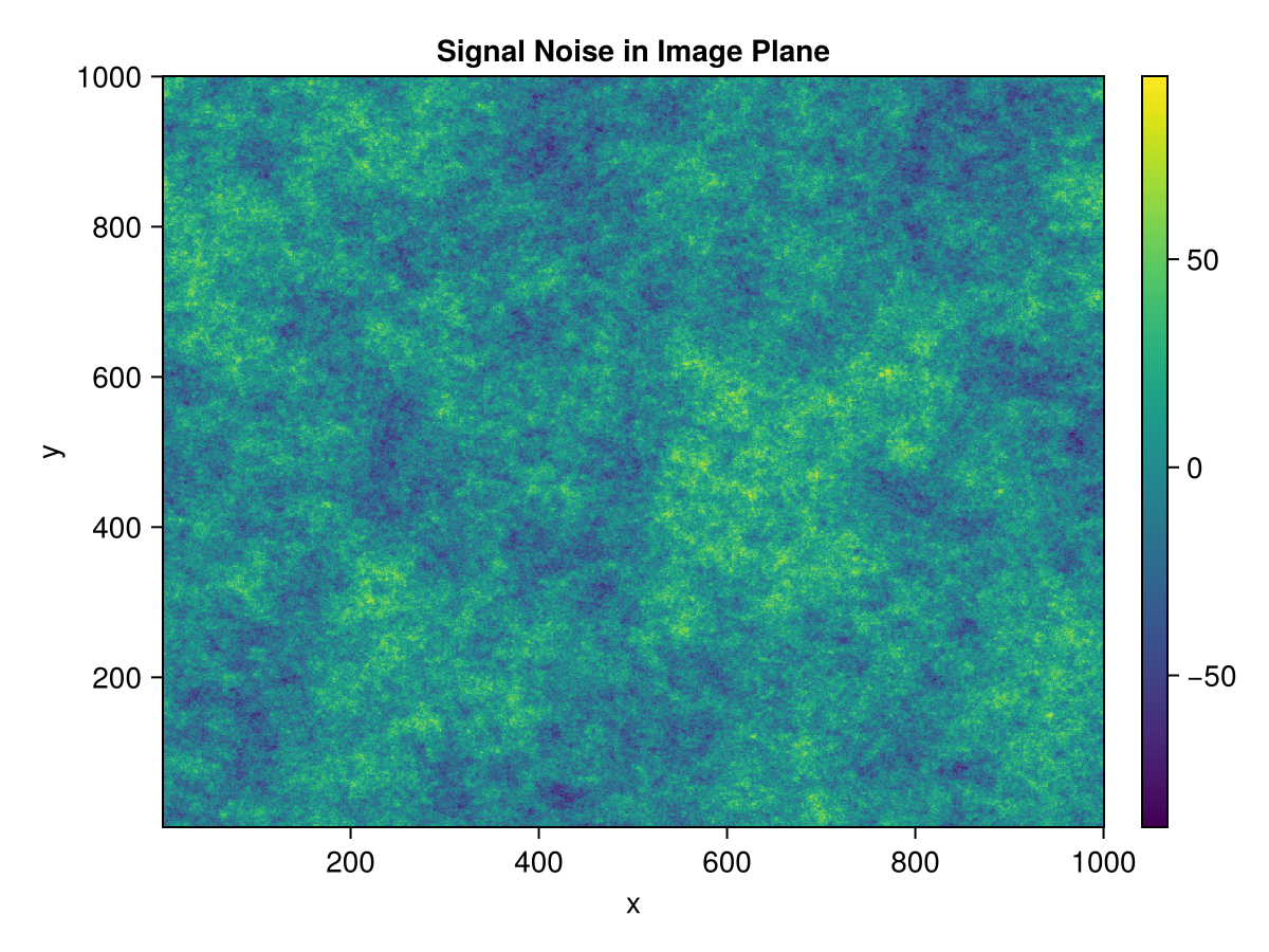
-7.92715 -3.05861 -18.3158 5.51787 -8.10642 -15.7977We can now plot our generated signal noise in the signal domain:
using CairoMakie

# plot signal noise in position plane
xgrid = (1:signal.dims[1],1:signal.dims[2])
fig = CairoMakie.Figure()
ax = Axis(fig[1,1], title = "Signal Noise in Image Plane", xlabel = "x", ylabel = "y")
cplot = CairoMakie.heatmap!(fig[1,1], xgrid..., signoise)
Colorbar(fig[1,2], cplot)
fig