Tutorial
This example code segment uses StationaryRandomFields.jl to generate correlated noise for a signal of given dimensions.
We begin by defining a noise signal object with dimensions input as a tuple.
using StationaryRandomFields
using FFTW

# Define a 2D signal with dimensions (1000,1000)
signal = NoiseSignal((1000,1000))
NoiseSignal{Tuple{Int64, Int64}}((1000, 1000))We can immediately access the RFFT frequency grid that corresponds to the signal dimensions
ν = rfftfreq(signal)([0.0, 0.001, 0.002, 0.003, 0.004, 0.005, 0.006, 0.007, 0.008, 0.009000000000000001 … 0.491, 0.492, 0.493, 0.494, 0.495, 0.496, 0.497, 0.498, 0.499, 0.5], [0.0, 0.001, 0.002, 0.003, 0.004, 0.005, 0.006, 0.007, 0.008, 0.009000000000000001 … -0.01, -0.009000000000000001, -0.008, -0.007, -0.006, -0.005, -0.004, -0.003, -0.002, -0.001])We can also directly create Gaussian noise in Fourier space for the given signal with an optional input of the desired rng (if not the default). This is not a necessary step as the NoiseGenerator will implement it automatically later.
gnoise = generate_gaussian_noise(signal)501×1000 Matrix{ComplexF64}:
0.0+0.0im 0.025053+0.376979im … 0.292487-0.96599im
1.24881-0.107214im 0.571057-0.472652im 0.384168-0.0516825im
0.422543+0.414898im -0.0892877+0.240646im 1.1079-0.55863im
-0.895205+0.461682im 1.14372-0.526489im -0.788269-1.08733im
0.40204-0.609452im -0.165674+0.421465im 0.169188-0.237103im
0.486144-0.139198im -0.570832+0.0759267im … -1.12476-0.77402im
1.37852-0.417852im -0.121298-0.18023im 0.336492-1.93366im
0.512966-1.59188im 0.905531+0.151393im 0.283328+0.776298im
0.442851-0.215881im -0.106834+0.627754im 0.72668+0.408696im
0.475636+0.0118228im -0.149669-0.438577im 1.6296+0.384291im
⋮ ⋱
-0.52372+0.294498im 0.479387+0.11843im -0.0187201-0.720394im
0.395324+0.265344im -0.437361+0.738118im -1.75934+0.336355im
-0.18345-1.32786im 0.0844448+0.43262im 0.183757+0.850039im
1.40305+0.508264im -0.429878+0.207354im … -0.476452-0.165538im
-0.00686906+1.72325im 0.868014+0.919652im -0.0011277-0.0667045im
-1.64015+0.83224im 0.102208-1.16884im -0.31631-0.360008im
0.401063+1.11725im -0.375706-0.552955im -0.185285-0.0942509im
0.397389+0.644382im -0.0539036-0.993886im -0.121578-0.112911im
-0.702134+0.0im 0.645532-1.27461im … 1.31129-0.64632imNow construct the power spectrum to be used, designating the dimension in brackets.
# Create a basic power spectrum with index β = -2
ps = SinglePowerLaw{2}(-2.)
SinglePowerLaw{2, Float64}(-2.0)The power spectrum may be modified via renormalization, rotation, and stretching
renormed_ps = 1000 * ps
rotated_ps = rotated(renormed_ps, π/6) # π/6 is the rotation factor
stretched_ps = stretched(rotated_ps, 100, 100) # 100 is the stretch factor of both axes
ModifiedPowerSpectrumModel
base model: SinglePowerLaw{2, Float64}
Modifiers:
1. Renormalize{Int64}
2. Rotate{Float64}
3. Stretch{Int64, 2}The noise generator requires a ContinuousNoiseSignal as input, which can be created from the original NoiseSignal
cns = ContinuousNoiseSignal(signal)ContinuousNoiseSignal{Float64, NoiseSignal{Tuple{Int64, Int64}}, Tuple, FFTW.rFFTWPlan{Float64, -1, false, 2, Tuple{Int64, Int64}}, AbstractFFTs.ScaledPlan{ComplexF64, FFTW.rFFTWPlan{ComplexF64, 1, false, 2, Tuple{Int64, Int64}}, Float64}}(NoiseSignal{Tuple{Int64, Int64}}((1000, 1000)), (1000, 1000), FFTW real-to-complex plan for 1000×1000 array of Float64
(rdft2-rank>=2/1
(rdft2-vrank>=1-x1000/1
(rdft2-ct-dit/20
(hc2c-direct-20/76/0 "hc2cfdftv_20_avx2"
(rdft2-ct-dit/2
(hc2c-direct-2/4/0 "hc2cfdftv_2_avx2"
(rdft2-r2hc-direct-2 "r2cf_2")
(rdft2-r2hc01-direct-2 "r2cfII_2"))
(dft-direct-10 "n1fv_10_avx2_128"))
(rdft2-r2hc01-direct-20 "r2cfII_20"))
(dft-vrank>=1-x10/1
(dft-ct-dit/5
(dftw-direct-5/4 "t3fv_5_avx2_128")
(dft-direct-10-x5 "n2fv_10_avx2_128")))))
(dft-buffered-1000-x32/501-6
(dft-vrank>=1-x32/1
(dft-ct-dit/25
(dftw-direct-25/8 "t3fv_25_avx2_128")
(dft-vrank>=1-x25/1
(dft-ct-dit/5
(dftw-direct-5/4 "t3fv_5_avx2_128")
(dft-direct-8-x5 "n2fv_8_avx2_128")))))
(dft-r2hc-1
(rdft-rank0-tiledbuf/2-x32-x1000))
(dft-buffered-1000-x21/21-6
(dft-vrank>=1-x21/1
(dft-ct-dit/25
(dftw-direct-25/8 "t3fv_25_avx2_128")
(dft-vrank>=1-x25/1
(dft-ct-dit/5
(dftw-direct-5/4 "t3fv_5_avx2_128")
(dft-direct-8-x5 "n2fv_8_avx2_128")))))
(dft-r2hc-1
(rdft-rank0-tiledbuf/2-x21-x1000))
(dft-nop)))), 1.0e-6 * FFTW complex-to-real plan for 501×1000 array of ComplexF64
(rdft2-rank>=2/1
(rdft2-vrank>=1-x1000/1
(rdft2-ct-dif/20
(hc2c-direct-20/76/0 "hc2cbdftv_20_avx2"
(rdft2-ct-dif/2
(hc2c-direct-2/4/0 "hc2cbdftv_2_avx2"
(rdft2-hc2r-direct-2 "r2cb_2")
(rdft2-hc2r10-direct-2 "r2cbIII_2"))
(dft-direct-10 "n1bv_10_avx2_128"))
(rdft2-hc2r10-direct-20 "r2cbIII_20"))
(dft-vrank>=1-x10/1
(dft-ct-dit/5
(dftw-direct-5/4 "t3bv_5_avx2_128")
(dft-direct-10-x5 "n1bv_10_avx2_128")))))
(dft-buffered-1000-x32/501-6
(dft-vrank>=1-x32/1
(dft-ct-dit/25
(dftw-direct-25/8 "t3bv_25_avx2_128")
(dft-vrank>=1-x25/1
(dft-ct-dit/5
(dftw-direct-5/4 "t3bv_5_avx2_128")
(dft-direct-8-x5 "n2bv_8_avx2_128")))))
(dft-r2hc-1
(rdft-rank0-tiledbuf/2-x32-x1000))
(dft-buffered-1000-x21/21-6
(dft-vrank>=1-x21/1
(dft-ct-dit/25
(dftw-direct-25/8 "t3bv_25_avx2_128")
(dft-vrank>=1-x25/1
(dft-ct-dit/5
(dftw-direct-5/4 "t3bv_5_avx2_128")
(dft-direct-8-x5 "n2bv_8_avx2_128")))))
(dft-r2hc-1
(rdft-rank0-tiledbuf/2-x21-x1000))
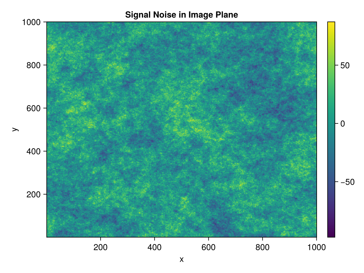
(dft-nop)))))Now create a power spectrum noise generator comprising the designated power spectrum and continuous noise signal. Note that the power spectrum and noise signal must be of the same dimension. The output signoise gives correlated power-law noise in the signal domain, with dimensions of the original NoiseSignal object.
noisegen = PSNoiseGenerator(stretched_ps, cns)
# generate signal noise
signoise = generate_signal_noise(noisegen)
1000×1000 Matrix{Float64}:
-20.5302 -16.3262 -14.1909 … -3.02384 -3.10226 -14.9543
-27.363 -19.1741 -15.9605 -3.44117 -3.25869 -14.1378
-2.75085 -12.6603 1.88619 -19.1302 -20.5177 -13.6973
-19.4876 10.7096 -0.384243 -30.488 -24.0301 -14.8945
-18.6332 9.10993 -3.33145 -17.0091 -16.8739 -10.5398
-3.41196 19.477 8.47633 … 1.26564 2.13773 -0.112194
15.913 22.819 20.8777 -19.8515 -4.30997 9.54119
24.3207 15.9159 9.74647 -1.62457 -3.81995 3.62966
-8.76021 5.23261 5.48984 15.3815 -0.894264 -15.2926
-16.9863 -5.86662 -2.31127 -6.85616 -1.57343 -7.84689
⋮ ⋱
-20.1375 -13.4466 5.53159 -14.1821 -2.77981 -7.71628
-32.4938 -18.9255 -15.7048 -35.6264 -6.47342 -11.507
-23.1447 0.116035 -1.99389 -25.2033 -2.42517 -14.4286
-7.77965 15.6969 3.69741 -14.5065 9.59357 -5.75431
0.859819 -20.7109 -25.1462 … 3.89705 6.33158 -3.35659
-4.16308 -3.65596 -28.546 4.05581 0.36165 -1.98395
2.62107 -12.6047 -26.345 -3.64691 -10.9994 -5.24013
-6.10264 1.80031 3.95277 -2.32892 -3.86726 -9.45356
-18.0786 -12.641 6.51464 0.9873 -12.3535 -19.8396We can now plot our generated signal noise in the signal domain:
using CairoMakie

# plot signal noise in position plane
xgrid = (1:signal.dims[1],1:signal.dims[2])
fig = CairoMakie.Figure()
ax = Axis(fig[1,1], title = "Signal Noise in Image Plane", xlabel = "x", ylabel = "y")
cplot = CairoMakie.heatmap!(fig[1,1], xgrid..., signoise)
Colorbar(fig[1,2], cplot)
fig